Baysian Inference Election Forecasting

Election forecasting caught my attention during the 2012 election cycle while I was a mathematics undergraduate student at The University of Texas at Austin. My statistics professor brought Nate Silver’s blog, FiveThirtyEight, into the classroom, and I have followed the blog ever since. I had not thought of trying to create my own model until learning about Bayesian Inference this semester in Dr. White’s Advanced Probability and Statistics class. While we only briefly touched on the subject, Dr. White brought up the example of Silver’s model, and gave an overview of how the model used Bayesian methods to forecast the probability of a given candidate’s victory. At the same time as Bayesian Inference was being introduced by Dr. White, we began discussing the modeling project in Math Modeling.

Bayesian statistics appealed to me because it fits my intuition more than a frequentist approach. In Bayesian inference, the statistician records some prior belief, collects data, and updates their belief accordingly. Where the frequentist sets a number of trials, the Bayesian can continue collecting more and more data as it becomes available. The Bayesian feeds the results of the previous data analysis as a new prior belief and repeats the process. Likewise, the interpretation of bounding reasonable values is more straightforward. For example, if I wanted to create a bound based on alpha = .05, the frequentist statistician creates confidence intervals and claims that if they repeated this process of creating intervals many times over, they would find that the true value lies within 95% of the intervals created. The Bayesian interpretation is that the true value has a 95% chance of being in the interval; no need to discuss the simulation of creating the intervals over and over again.

I used Bayesian Inference to examine a potential Trump vs. Biden general election battle. The model simplified reality, treating every state as a winner-take-all binary outcome, overlooking partial systems like Maine and Nebraska, and ignoring any third party candidates. Data came from two sources. For the larger data set, I looked at old presidential election data for each state from MIT election data and compared the number of votes each historic candidate received. If the state had more votes for the Democrat than it did for the Republican, a success would be recorded. Otherwise, a failure would be recorded. Likewise, for the smaller data set, I looked at current polls from Real Clear Politics and once again compared totals. The only polls considered were Biden vs. Trump, no other potential democratic nominee’s polls influenced the model.

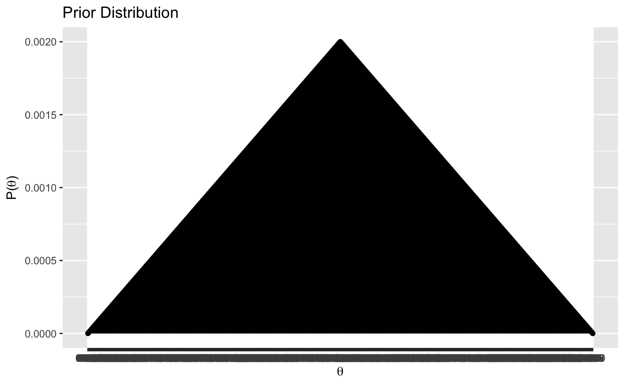
For each state, I generated a prior triangular distribution centered on 0.50, then I brought in both the large and small data sets to build likelihood distributions. Later, a compromise is reached between the likelihood and prior distributions, resulting in a posterior distribution. Once all this is done, I can easily find the most likely value for the probability of the state committing its electoral college votes to Biden, but I need to consider all of the credible values of the probability and I created an interval that contains those most credible values. Finally, the last step was to create a unified prediction of Biden’s chance to win the election overall. To accomplish this, I simulated different outcomes for each state, built a probability distribution and summed up the area under the curve to the right of 270. This resulted in the probability that Biden has more than 270 electoral college votes.

I used a triangular distribution over the uniform distribution as my prior since my limited knowledge on the subject suggested that 0.5 is the most likely probability, and as we move away from this center the probability decreases.

get_prior_distr <- function(vals) {
  vals_pmin <- pmin(vals, 1 - vals)
  # Normalize the prior so that they sum to 1.
  tibble::tibble(theta = vals, prior = vals_pmin / sum(vals_pmin)
  )
}

After creating my prior, I collected data by accessing past election results from MIT election data and polling information from Real Clear Politics and created likelihood distributions for each state.

get_likelihood_df <- function(theta_vals, num_succss, num_fails) {
  likelihood.vals <- c()
  for (cur.theta.val in theta_vals) {
    likelihood.vals <- 
      c(likelihood.vals, 
        (cur.theta.val^num_succss) * (1 - cur.theta.val)^(num_fails))
  }
  likelihood.vals <- dbinom(num_succss, num_succss + num_fails, theta_vals)
  likelihood_df <- 
    tibble::tibble(
      theta = theta_vals,
      likelihood = likelihood.vals
    )

  return(likelihood_df)
}

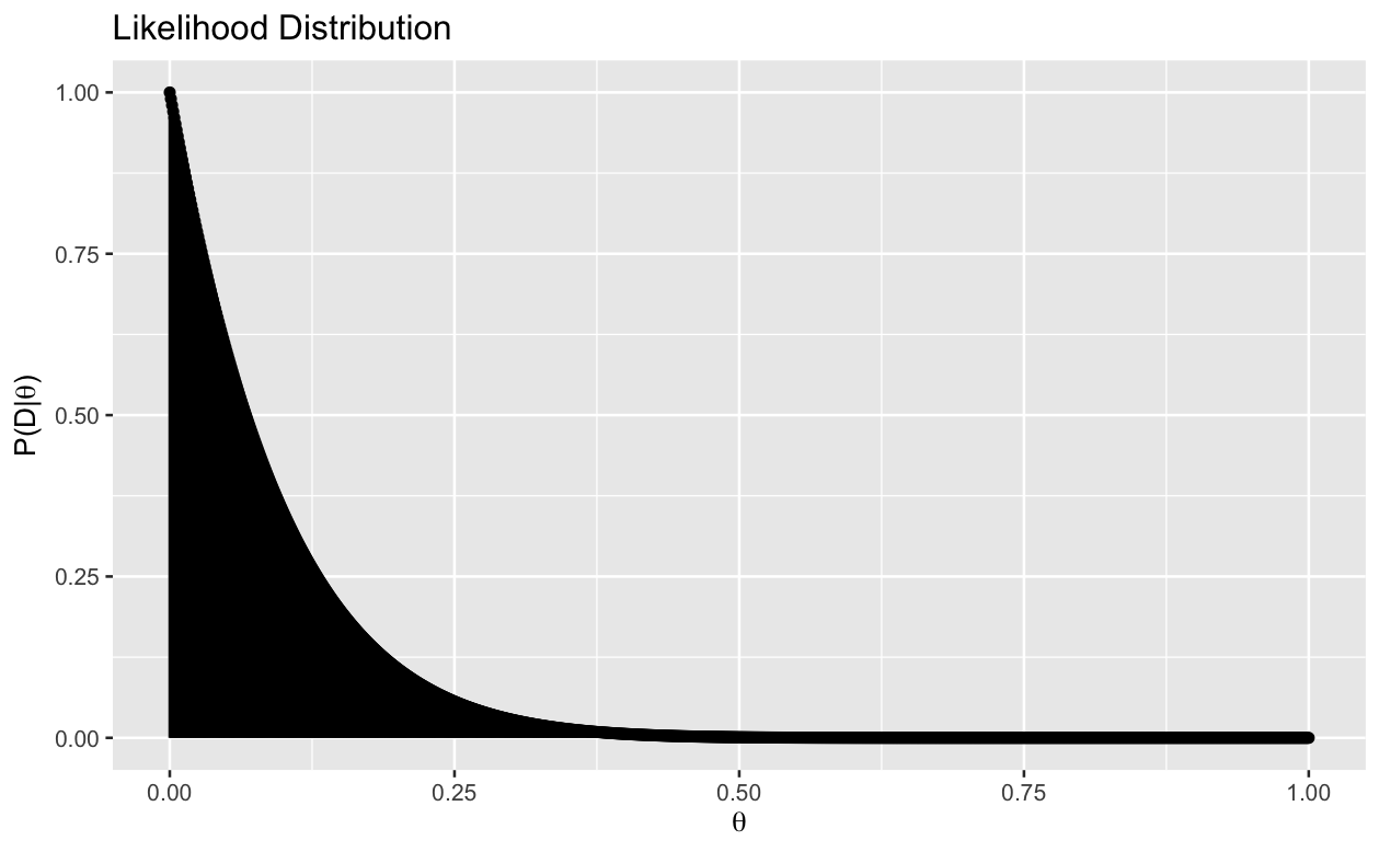
The likelihood distribution was created by taking each theta value and computing its likelihood value. Next, I calculate the posterior distribution the marginal likelihood found by finding the likelihood at every possible theta value and summing them up.

get_posterior_df <- function(likelihood_df, prior_distr_df) {

  likelihood_prior_df <- dplyr::left_join(likelihood_df, prior_distr_df, by = "theta")

  marg_likelihood <- likelihood_prior_df %>%dplyr::mutate(likelihood_theta = .data[["likelihood"]] * .data[["prior"]]) %>% dplyr::pull("likelihood_theta") %>%sum()

  posterior_df <- dplyr::mutate(likelihood_prior_df, post_prob = (likelihood * prior) / marg_likelihood)

  return(posterior_df)
}

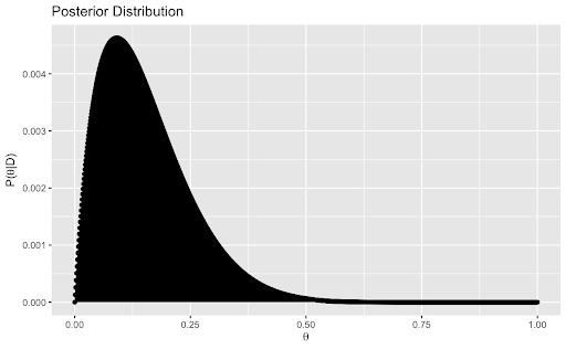
At this point, I have found the posterior distribution of theta. Next, I add a credibility interval to find a reasonable range for where theta could be. This credible range is defined as a and b such that

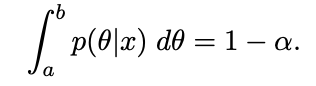
where alpha is the level of significance, a represents the lower bound, and b is an upper bound. I accomplished this using a function ci() adapted from user submitted answers on stats.stackexchange.com.

ci <- function(x, px){  # Function created using https://stats.stackexchange.com/questions/240749/how-to-find-95-credible-interval

  xx <- seq(min(x), max(x), by = 0.05)

  # interpolate function from the sample
  fx <- splinefun(x, px) # interpolating function
  pxx <- pmax(0, fx(xx)) # normalize so prob >0

  # sample from the "empirical" distribution
  samp <- sample(xx, 1e5, replace = TRUE, prob = pxx)

  # and take sample quantiles
  quantile(samp, c(0.025, 0.975)) 

  cpxx <- cumsum(pxx) / sum(pxx)
  xx[which(cpxx >= 0.025)[1]]   # lower boundary
  xx[which(cpxx >= 0.975)[1]-1] # upper boundary

  return(c(xx[which(cpxx >= 0.025)[1]],xx[which(cpxx >= 0.975)[1]-1]))   # lower boundary, upper

which hacks its way around some computational limits using sampling. Note that in the function used, alpha is 0.05. I repeated this process for every state, and graphed the results. The data point was placed for the theta value that has the highest probability of occuring, and the error bars extend to the end of the 95% credibility interval.

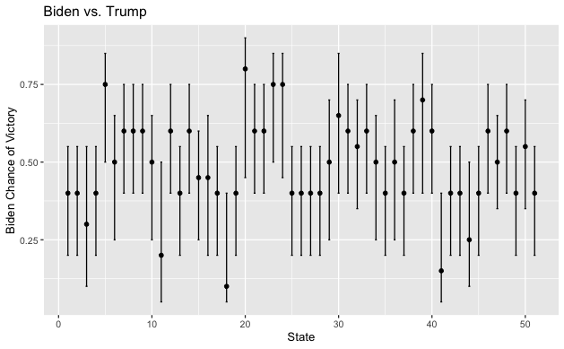
Clearly my model has significant variance and I am not certain of much. Based on this graph, it is unclear what Biden’s chances of winning are and it is even unclear if Biden or Trump have a higher probability of being elected.

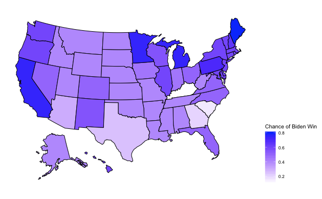
We get a little more information from a picture of the data mapped to the united states, but we are still lacking any input on the number of electoral college votes each state gets.

What I need is some sort of summary value that best captures who is going to win. I want something related to the expected number of votes that Biden will receive. Normally, expected value is calculated by taking each outcome and multiplying it by its probability, but in my Bayesian model, each probability has a probability associated with it. I ended up dealing with this by choosing random samples from the posterior probability of each state weighted by the probability of that probability occurring, taking that value and multiplying by the total number of electoral college votes for that state, and them summing up to find the total number of electoral college votes that Biden won from all the states combined. Doing this all the way through provided one simulation. I simulated this election one thousand times and build a density curve.

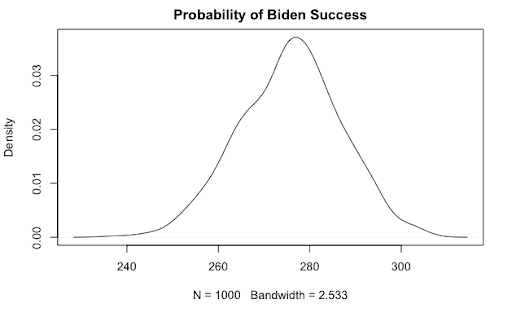
The density curve gave me a graphical depiction of what is likely to happen in the 2020 election. Based on the graph, the more area under the curve to the right of a given x value, the higher the probability of that many electoral college votes. Patterns can already be made out. The important value in this graph is 270, which is the number of votes that a candidate needs to overcome inorder to achieve a majority and be elected. The curve is centered to the right of 270, so based on the picture alone, the model is predicting that Biden is more likely to win than Trump. I still want a number that summarizes the model. To find the probability that Biden gets more than 270 electoral college votes I summed up the area under the curve to the right of 270. I found 0.706, or a 70.6% chance Biden wins under these conditions.

I had to step out of my comfort zone to build this model. I learned about Bayesian Inference this year, however we only briefly touched on it and discussed the differences between Frequentist and Bayesian statistics. We did not calculate any credibility intervals or look at large data sets. While I have used R before, I did not move beyond calculations until this project and I had never worked with a large dataset in any programming language before. I am thrilled to have a working model that I can add more to and update as new polls are added. As of December 10th, there are less than 15 states that have state level polling information, and there are only a handful of nationwide polls. The first thing I want to work on is the automation of pulling new polling data. Currently, I input the data manually for each poll. R already has libraries that support getting data from web pages, but it was another new topic to learn that I eventually cut from my project so that I could be sure to have a working prediction. Once web scraping is working, I want to turn that tool onto fivethirtyeight.com and scrape pollster rankings. I want to use these rankings to weight the effects that the polling data has on my model. That way, a high quality poll will have a larger effect than a poll that has more error or bias.

As I update my model and we get closer to the 2020 election, I hope to compare my results with other election forecasters such as the aforementioned fivethirtyeight, 270towin, and votamatic. Long term, fivethirtyeight has a blog post about self assessment over multiple predictions that I plan on working through. I need to learn about and make calibration plots and skill scores. Calibration plots will help me determine if things that I predict with a given percentage actually occur with that percentage and skill scores compare my prediction vs some sort of a set guess, like every candidate has the same probability of winning. As it stands, I do not have enough information to assess my forecasts, but since this model is in a working state, I can continue to update it for any election that I am interested in, creating more and more data that I can use to assess the validity of my model.